Home > Blogs > Input Shaping for Motion Control Vibration Reduction

Input Shaping for Motion Control Vibration Reduction

Background

Vibration reduction is crucial for many motion control applications. While this is obvious for applications like cranes where a swinging load will result in disaster or labs where a sloshing liquid will spill on expensive equipment, vibration reduction is equally important for high-precision motion control applications like imaging and inspection. Many objects that appear stiff are surprisingly flexible at the micron level. For applications like microscopy where minute vibrations will result in a blurry image, waiting for vibrations to decay can significantly increase the overall time it takes to perform a move.

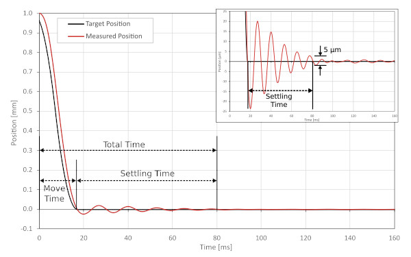
In motion control, settling time is defined as the time required for an axis’s measured position to remain within an acceptable tolerance of the target position after a motion trajectory finishes execution. In practice, settling time is often spent waiting for vibrations to decay. Because the total move time consists of the trajectory and settling time combined, a slower trajectory can often actually improve throughput because the vibrations (and thus settling time) decrease more than the trajectory time increases.

Input shaping is the theory of intentionally modifying system inputs to produce a desired system output. In motion control, input shaping refers to modifying the target motion trajectory to minimize vibrations. This article presents various input shaping techniques that can be used on almost any motion controller to reduce vibrations and decrease settling time.

Theory

Decreasing acceleration to reduce vibrations is the most basic form of input shaping. It is intuitive that decreasing acceleration will typically reduce vibrations, but how does this work? The key is that acceleration is directly proportional to the magnitude of inputs (in our case forces) on the system via Newton’s second law: F=ma. For linear systems, the output is directly proportional to the magnitude of the applied input, so the vibration amplitude will decrease proportionally.

However, it is important to note from control theory that system outputs (vibrations) depend on the magnitude and frequency of inputs. This relationship can be shown on a bode plot, where system outputs are plotted over a range of input frequencies.

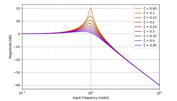
All underdamped systems have a resonant frequency where the inputs (forces) will be drastically multiplied to produce large outputs (vibrations). The resonant frequency appears as a sharp peak on the bode plot. While this peak can be reduced by adding damping to the system or decreasing the magnitude of inputs, it is ideal to move the frequency of inputs away from the resonant frequency.

To minimize vibrations, the frequency content of accelerations and decelerations in a motion trajectory should be as far away from the system’s resonant frequency as possible.

Zero Vibration Shaping

For systems with one resonant frequency, it is possible to exploit the frequency dependence of inputs such that a trajectory can completely cancel out its own vibration. Input shaping algorithms that fully cancel out vibration at a specific frequency are known as zero vibration (ZV) shapers.

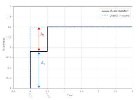
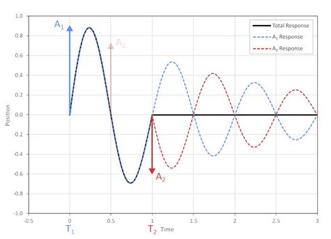
One method^[1] for ZV shaping works by calculating two impulses, offset by half the vibration period, which result in zero vibration (figure 3a). These impulses can be convolved with any motion trajectory to produce a modified trajectory which will also result in zero vibration. When implemented for a trapezoidal velocity motion profile as shown in figure 3b, the basic process is to:

Split the original acceleration into two fractions, A₁ and A₂.
Start accelerating at rate A₁.
Wait for half the vibration period.
Increase the acceleration to rate A₁ + A₂.

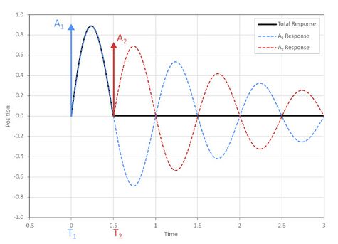
This shaping process splits the acceleration into two phases, where the second phase cancels out the vibration created by the first. The downside to this algorithm is that a move time penalty of half the vibration period is incurred. However, the elimination of vibrations and thus reduction in settling time means that there is usually a net performance boost even with the increased trajectory time.

A Generic ZV Algorithm

There are many input shaping methods that have been researched and implemented for vibration reduction in motion control applications. These algorithms vary in complexity and can include features such as the ability to target multiple resonant frequencies, or insensitivity to vibration characterization errors. However, all these algorithms, including the one presented above, require specialized firmware level algorithms to split acceleration into many precisely timed phases. Since the purpose of this article is to discuss general vibration reduction methods which can be implemented on most standard motion controllers, including Zaber’s X-Series controllers, this problem can be simplified by assuming:

The total distance of the movement is known beforehand.
Vibration during the move doesn’t matter, only after stopping.

These two assumptions allow us to simplify the shaping algorithm. Impulse A₂ is negated and executed after one full vibration period instead of a half period. This key change creates a trajectory in which the deceleration cancels out the vibration induced by the acceleration. The process is now:

Start accelerating at rate A₁.
Wait one full vibration period – this is controlled by adjusting the trajectory max speed.
Start decelerating at rate A₂ – deceleration is slower than acceleration because the vibration from A₁ will have decayed slightly by the time deceleration starts.

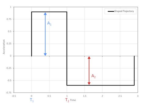
This is a simple trajectory that can be implemented on any motion controller supporting trapezoidal velocity profiles where acceleration, deceleration, and max speed can be adjusted. It should also be noted that deceleration can start at any n number of full vibration periods after the acceleration starts, but the magnitude must be decreased by the accordingly by the vibration decay rate.

Equations

The equations for the input shaping algorithm are derived from reference [1] and basic damped vibration theory. A calculator spreadsheet is also provided for simplicity.

First, we define a dimensionless vibration decay factor K, which is given by

where,

ζ is the vibration damping ratio [-]
n is the integer number of vibration periods between impulses [-]

From ZV input shaping theory, the times and amplitudes of each impulse are given by:

(2a)

(3a)

(2b)

(3b)

where,

T_i is the time when each impulse is executed [s]
A_i is the magnitude of each impulse [-]
f is the vibration resonant frequency [Hz]

Because only the relative magnitude of each impulse is important, we can define the deceleration based on the ratio of impulses and magnitude of acceleration:

where,

a is the trajectory acceleration [m/s²]
a_d is the trajectory deceleration [m/s²]

Deceleration should be started at the time for the second impulse, hence from 2b

where,

T_d is the time to begin deceleration [s]

The following equations determine the trajectory parameters required to satisfy the above conditions for zero vibration. They are derived from constant acceleration equations for a trapezoidal velocity profile trajectory (figure 5).

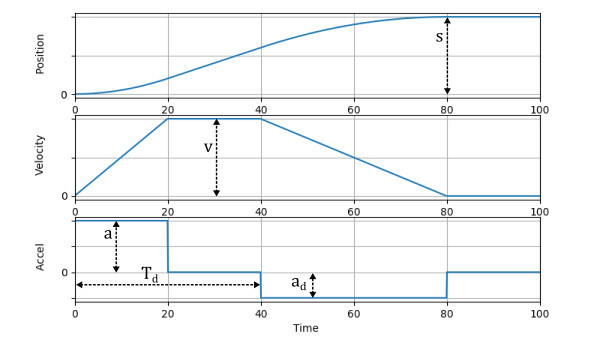
The trajectory max speed required to begin decelerating at the correct time can be found by solving for the roots of equation 6:

where,

v is the trajectory max speed [m/s]
s is the trajectory distance [m]

Equation 7 defines the slowest possible acceleration that can still reach the deceleration point at the correct time:

where,

a_min is the minimum trajectory acceleration [m/s²]

If a device is not capable of the acceleration a_min or velocity v, the value of n can be increased until these trajectory limits are feasible. However, for optimal performance it is ideal to n as low as possible.

A Practical Example

An X-ADR series microscope stage was used to demonstrate a practical example of the zero-vibration input shaping algorithm. The general procedure is to:

Perform a representative movement and measure the vibration.
Characterize the resonant frequency and damping ratio of the vibration.
Apply the input shaping theory to calculate new trajectory parameters.
Perform a movement with the optimized trajectory parameters.
Tweak the resonant frequency and damping ratio slightly as needed to account for modelling errors.

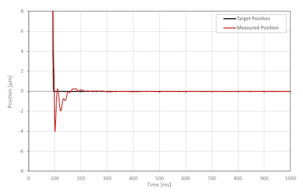
The stage was placed on a typical office desk and commanded to execute a 1 mm move. The dataset in figure 6 shows the stage’s final position approach and was captured from the onboard 1 nm resolution encoder. Although the target trajectory executes in 53 ms, there is a precise vibration that continues for over 1000 ms.

This result demonstrates how an object that appears stiff like a sturdy office desk can severely limit throughput for high precision applications. For imaging applications, it is required to wait until the vibration amplitude is less than the size of one pixel to take a sharp image. For a pixel size of 1 µm, this vibration would require waiting for around 1 second.

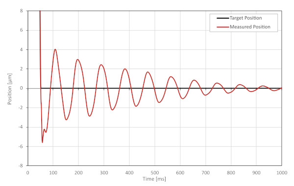
From the measured position in figure 6, a resonant frequency of 11.0 Hz and damping ratio of 0.046 can be approximated. While the best way to estimate these parameters is to plot a theoretical vibration decay on top of the dataset and adjust the parameters until it matches well, the parameters can also be quickly estimated from any two vibration peaks on the graph by the following equations:

where,

f is the resonant frequency [Hz]
ζ is the damping ratio [-]
T₀ and T_n is the time at peaks zero and n, respectively [s]
X₀ and X_n is the amplitude of peaks zero and n, respectively [µm]
n is the number of peaks between peak zero and peak n [-]

The approximated frequency and damping ratio are then fed into the input shaping calculator to determine a modified trajectory which will cancel out the specified vibration. The original and shaped trajectories are shown in table 1 and figure 7. The input shaping algorithm has adjusted the max speed to ensure that deceleration starts exactly one vibration period after motion starts (91ms). The algorithm has also increased the deceleration to match the magnitude of the decaying vibration at that time

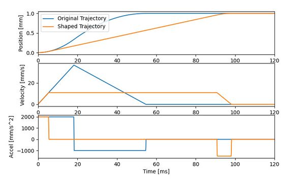
Trajectory	Original	Shaped	Zaber Setting
Distance [mm]	1	1	–
Max Speed [mm/s]	250	10.9	maxspeed
Acceleration [mm/s2]	2000	2000	motion.accelonly
Deceleration [mm/s2]	1000	1497.5	motion.decelonly
Execution Time [ms]	53	98	–

Table 1: Trajectory parameters for both datasets captured in this example.

The dataset in figure 8 was captured immediately after the first but with the shaped trajectory parameters. The comparison is remarkable; the vibration is almost completely non-existent, and the stage settles nicely after 250ms. While the shaped trajectory takes 45 ms longer to execute, the reduction of vibration decreases the total movement and settling time by 750 ms. Simply adjusting the trajectory has resulted in a throughput increase of over 4x!

There may still be residual vibration remaining after applying the input shaping. This could indicate errors in the approximated resonant frequency or damping ratio. In this scenario, it is recommended to try adjusting these values slightly and re-running the experiment to see if the vibration can be reduced further.

Practical Limitations

There are some limitations to be aware of with the input shaping theory presented in this article:

The motion will always take as long as one vibration period plus deceleration time.

Because deceleration needs to start after exactly one (or more) full vibration periods, a fundamental limit is placed on the minimum trajectory time. This means the trajectory can take a very long time for systems with a low resonant frequency. The same goes for systems with high damping ratios, as the deceleration may be very slow even if the acceleration is fast. The latter is not as much of a problem though, because vibrations with a high damping ratio decay quickly regardless of input shaping.

The system must have only one dominant resonant frequency, for which the resonant frequency and damping ratio can be estimated with reasonable accuracy.

The input shaping algorithm presented in this article can only mitigate one resonant frequency. For systems with multiple resonant frequencies (ex. a liquid sample on a wobbly table), only one of these frequencies can be compensated for.

Additionally, zero vibration shapers only fully cancel vibration if the resonant frequency and damping ratio estimates are perfect. In practice there will always be some error in these values, but it is ideal to be within a few percent of the actual values. If the frequency is off by more than 50%, the input shaping algorithm will actually start to amplify the vibration! Thankfully, the 1 nm resolution linear encoders on Zaber’s direct drive stages provide a very accurate tool for measuring vibration parameters.

The shaping algorithm may not work well if the trajectory takes significantly longer than the vibration period.

Consider the scenario where a stage is performing a long-distance move that takes many seconds. This may be enough time that the acceleration induced vibrations have completely died out and there is nothing left for the deceleration to cancel. In this case, increasing the speed of the stage so deceleration can start sooner should be considered. The effectiveness of the shaping algorithm depends on the vibration decay time relative to the stage’s ability to execute a trajectory in a certain time (acceleration and max speed). Although the algorithm is valid if the stage starts decelerating any number of full vibration periods after the move started, the shaped deceleration may be prohibitively slow if many periods have passed and the vibration has decayed significantly. Ideally, the stage should move fast enough that the deceleration can begin after exactly one vibration period.

Relation to Other Trajectory Modifications

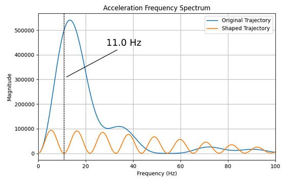
To minimize vibrations, it is important to accelerate and decelerate at a frequency that is far away from a system’s resonant frequency. Taking an FFT of the trajectory acceleration shows how this is achieved. Figure 9 shows the frequency spectrum of the shaped and unshaped accelerations from the previous example. This plot shows which frequencies the energy input into the system is distributed over. In this example, shaped trajectory has no energy at the target frequency of 11.0 Hz and higher harmonics. Although the energy from the motion must go somewhere, the shaping algorithm has shifted it away from the target frequency to other intermediate frequencies!

The idea of how input shaping shifts energy away from the system’s resonant frequency provides insight into how other modifications to the trajectory might influence system vibrations. For example: what if we decreased acceleration instead?

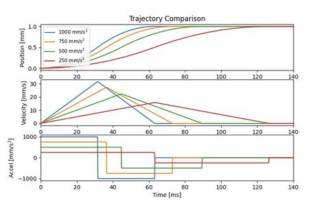
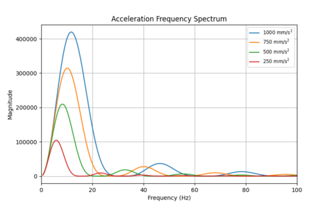
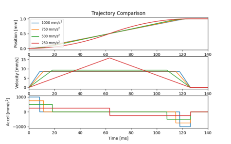
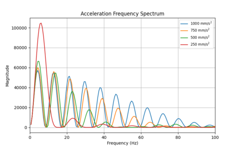
Figure 10b shows how the frequency spectrum changes when acceleration is decreased for an acceleration limited trajectory. Total energy decreases, which is expected because less energy is required for a slower move. The energy decrease is largest in the low frequency ranges, indicating that decreasing acceleration would likely be effective at reducing the 11.0 Hz vibration from the example above.

It should also be noted that decreasing acceleration shifts the large low frequency peak to even lower frequencies in addition to reducing its magnitude. In this case, decreasing the acceleration 4x shifts the peak frequency lower by approximately 2x.

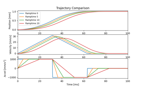
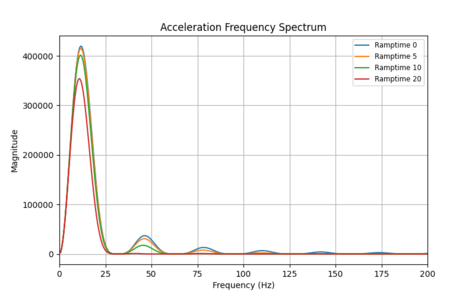
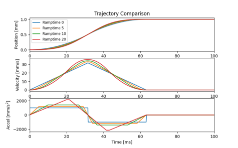
We can also experiment with the effect of jerk limiting using the motion.accel.ramptime setting. Figure 11b shows the impact of increasing the amount of jerk limiting while holding all other trajectory parameters constant.

As seen below, jerk limiting is very effective at removing higher frequency energy components but has almost no effect at low frequencies. For the example demonstrated in this article, jerk limiting would have almost no effect on the vibration at 11.0 Hz. It would only help if the resonant frequency was higher. This result also explains why jerk limiting is very effective at reducing higher frequency audible noise during motion

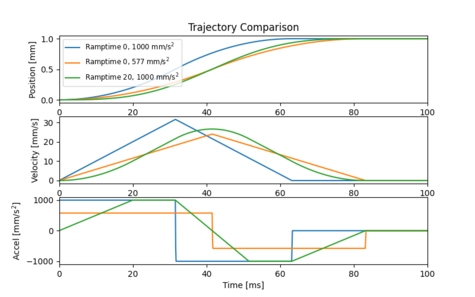
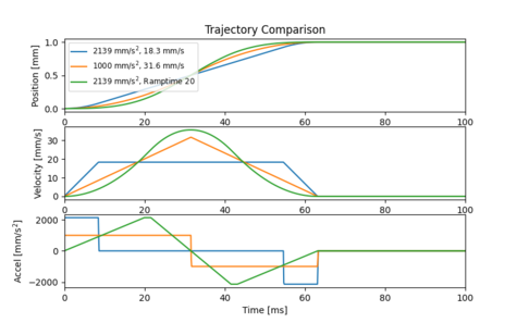
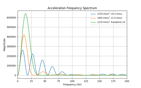
How do these two methods compare? Figure 12b shows the effect of increasing jerk limiting compared to decreasing acceleration such that each yields an equivalent 20 ms move time penalty. The result is clear; jerk limiting is best for reducing high frequency energy, while decreasing acceleration is best for reducing low frequency energy. Both methods also shift the primary peak to lower frequencies, but decreasing acceleration is far more effective at doing so.

The results above raise an important question: what if your application can’t tolerate a move time increase?

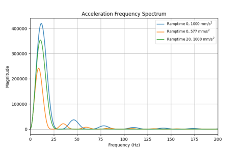
One option is to increase the maximum speed while decreasing acceleration so each move takes the same time. This comparison, shown in figure 13b, reveals an interesting trend. When a significant portion of the motion is spent at maximum speed, only decreasing acceleration is beneficial. High frequency energy is reduced with almost no change in low frequency energy. However, as the trajectory approaches pure acceleration, high frequency energy is shifted towards a single low frequency.

This result indicates that it is always beneficial to lower acceleration when a large portion of the trajectory is spent at maximum speed. However, once the trajectory is near the point of being acceleration limited, it is up to the user to choose whether they want the energy distributed over higher or lower frequencies.

A similar experiment is to increase jerk limiting while also increasing acceleration such that move time stays constant. From figure 14b we can see that jerk limiting has shifted energy from multiple higher frequencies towards a single low frequency.

This result makes intuitive sense because the acceleration profile begins to resemble a sine wave as jerk limiting is increased. However, it should be re-iterated that the low frequency energy increase means increasing jerk limiting will result in worse vibrations if the system’s resonant frequency is low.

If move time is kept constant, how does jerk limiting compare to decreasing acceleration? An example is shown in figure 15b with both decreased acceleration and jerk limiting, but where a constant move time is maintained by adjusting maximum speed.

Both options have similar results. Energy is shifted from high frequencies to lower frequencies. However, jerk limiting does so more aggressively; there is better high frequency reduction at the cost of a larger low frequency increase. In most applications, the ideal approach is to combine by methods by reducing acceleration until the low frequency components start to increase, then adding a small amount of jerk limiting to eliminate the remaining high frequency components.

A summary of the outcomes above is shown in table 2. It is worth noting that there isn’t necessarily one trajectory modification that is better than the others; it depends on the resonant frequency (or frequencies) of the system in question. One obvious exception to this rule is when a trajectory has very high acceleration and a long time spent at max speed; decreasing acceleration and increasing max speed will yield high frequency energy reduction with no move time increase.

Trajectory Modification	Result
Zero vibration shaping	Energy is strategically shifted away from target resonant frequencies. Move time may change.
Decreasing acceleration	Low frequency energy is decreased significantly. Energy is shifted towards lower frequencies. Move time increases.
Increasing jerk limiting	High frequency energy decreased significantly. Move time increases.
Decreasing acceleration. Constant move time by increasing speed.	High frequency energy is decreased, then gradually shifted to lower frequencies as trajectory approaches being acceleration limited.
Increasing jerk limiting. Constant move time by increasing acceleration or max speed.	High frequency energy is aggressively shifted to lower frequencies.