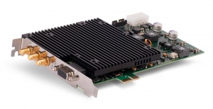
The TimeHarp 260 is a compact, easy to use, Time-Correlated Single Photon Counting (TCSPC) and Multi-Channel Scaling (MCS) board for the PCIe interface. It is based in a custom TDC design that offers an ultrashort dead time even at high temporal resolutions. The board is available in two versions with either 25 ps (PICO module) or 250 ps (NANO module) base resolution. The high quality and reliability of the TimeHarp 260 is expressed by a unique 5-year limited warranty.
Multiple input channels for highly flexible use
Each version of the TimeHarp 260 is available in different configurations with either one (SINGLE version) or two (DUAL version) independent detection channels and an additional common sync input. All of them, including the sync input, can be used as independent timing channels for coincidence correlation experiments. Alternatively the common sync input can be used for TCSPC with fast excitation sources. The other input(s) can then be used as independent detector channels for TCSPC. In this case the TimeHarp 260 allows forward start-stop operation at the full repetition rate of mode locked lasers with stable repetition rate up to 100 MHz.
PICO module for high resolution TCSPC
The TimeHarp 260 PICO is designed for high timing resolution. With a digital resolution of 25 ps and a timing jitter < 20 ps it is well matched to the timing resolution of the majority of common photon detectors. All input channels are equipped with software-adjustable Constant Fraction Discriminators (CFD) sensitive on the falling edge. The ultra short dead time of the TimeHarp 260 PICO of < 25 ns per channel allows very high measurement rates. Along with the extremely low differential non-linearity of the instrument, excellent data quality can be obtained.
The histogramming time range of the TimeHarp 260 PICO can be extended up to seconds with an optional “long range mode”. In this mode the base resolution of the board is switched to 2.5 ns and the dead time reduces to < 2.5 ns. This permits to study dynamics from picoseconds up to seconds with just a single board.
NANO module for MCS and nearly deadtime-free correlation
The TimeHarp 260 NANO is designed for ultimately short dead time at a moderate time resolution. Exactly like the PICO model it can be used for coincidence correlations across all inputs or for TCSPC with light source trigger connected to the sync input. Because of the short dead time and the long histogram range it is particularly suited for classical Multi Channel Scaler (MCS) applications. Software-adjustable discriminators and polarity switches allow the TimeHarp 260 NANO to be interfaced to a wide range of signal and trigger sources. The board’s multi-stop capability allows efficient recording of long-lived fluorescence and luminescence decays up to the seconds time range with correspondingly slow excitation rates, yet at very high detector count rates.
Adjustable delay in each input channel
Each input channel has an internal adjustable delay with ±100 ns range at either 25 ps resolution (PICO model) or 250 ps resolution (NANO model). This unique feature eliminates the need for specially adapted cable lengths or cable delays for changes in experimental set-ups.
Operation as time tagger
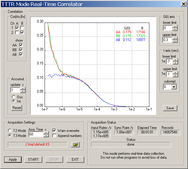
A Time-tagged mode for recording of individual photon events with their arrival time on all channels allows the most sophisticated offline analysis of the photon dynamics. Time-Tagged Time-Resolved (TTTR) data can also be correlated in real-time for monitoring of FCS experiments at count rates up to 1 000 000 counts/sec. External marker signals are supported by the versions with two detection channels and can be used to synchronize the device with other hardware such as scanners, e.g., for Fluorescence Lifetime Imaging (FLIM).
Programmable trigger out
The TimeHarp 260 also features a trigger output, which can generate pulse periodes between 0.1 µs and 1678 s, corresponding to repetition frequencies between 0.596 Hz and 10 MHz. This feature can, e.g., be used to control external lasers.
|
TimeHarp 260 PICO |
TimeHarp 260 NANO |
| Input channels and sync |
Constant Fraction Discriminator (CFD) on all inputs, software adjustable |
constant level trigger on all inputs, software adjustable |
| Number of detector channels (in addition to sync) |
1 (SINGLE) or 2 (DUAL) |
1 (SINGLE) or 2 (DUAL) |
| Input voltage range (pulse peak into 50 Ohms) |
0 to -1200 mV, optimum: -100 mV to -200 mV |
-1200 mV to +1200 mV |
| Input voltage max. range (damage level) |
±1500 mV |
±2500 mV |
| Trigger edge |
falling edge |
falling or rising edge, software adjustable |
| Trigger pulse width |
0.5 to 30 ns |
> 0.5 ns |
| Trigger pulse required rise/fall time |
2 ns max. |
— |
| Time to Digital Converters |
| Minimum time bin width |
25
in optional “long range mode”: 2.5 ns ps |
250 ps* |
| Timing precision** |
< 20 ps
in optional “long range mode”: < 1 ns rms rms |
< 250 ps rms* |
| Timing precision / √2** |
< 14 ps rms
in optional “long range mode”: < 710 ps rms |
< 180 ps rms* |
| Dead time |
< 25 ns
in optional “long range mode”: <2.5 ns |
< 2 ns |
| Peak count rate per input channel |
40 × 106 counts/sec
in optional “long range mode”: 400 × 106 counts/sec for bursts of up to 128 events |
1000 x 10^6 counts/sec for bursts of up to 96 events |
| Sustained count rate per input channel |
40 × 106 counts/sec |
40 × 106 counts/sec |
| Maximum sync rate (periodic pulse train) |
100 MHz |
100 MHz |
| Adjustable delay range for each input channel |
±100 ns, resolution 25 ps |
±100 ns, resolution 250 ps* |
| Differential non-linearity |
< 2% peak, <0.2% rms (over full measurement range) |
< 2% peak, <0.2% rms (over full measurement range) |
| Histogrammer |
| Count depth |
32 bit (4 294 967 296 counts) |
32 bit (4 294 967 296 counts) |
| Maximum number of time bins |
32 768 |
32 768 |
| Full scale time range |
819 ns to 1.71 s (depending on chosen resolution: 25 ps, 50 ps, 100 ps, …, 52.42 µs)
in optional “long range mode”: 81.92 µs to 171 s (depending on chosen resolution: 2.5 ns, 5 ns, 10 ns, …, 5242 ms) |
8.19 µs to 17.1 s (depending on chosen resolution: 250 ps, 500 ps,…, 524.2 µs)** |
| Acquisition time |
1 ms to 100 hours |
1 ms to 100 hours |
| Sustained throughput (sum of all channels)*** |
typ. 30×106 events/sec (depending on host PC configuration and performance) |
typ. 30×106 events/sec (depending on host PC configuration and performance) |
| TTTR Engine |
| T2 mode resolution |
25 ps |
250 ps* |
| T3 mode resolution |
25 ps, 50 ps, 100 ps,…, 52.42 µs in optional „long range mode“: 2.5 ns, 5 ns, 10 ns, …, 5 242 ms |
250 ps, 500 ps, 1 ns, …, 524.2 µs* |
| FiFo buffer depth (records) |
8 388 608 |
8 388 608 |
| Acquisition time |
1 ms to 100 hours |
1 ms to 100 hours |
| Sustained throughput (sum of all channels)*** |
typ. 40×106 events/sec |
typ. 40×106 events/sec |
| Trigger Output |
|
only available along with optional long range mode |
always enabled |
| Period |
programmable, 0.1 µs to 1678 s (0.596 Hz to 10 MHz) |
programmable, 0.1 µs to 1678 s (0.596 Hz to 10 MHz) |
| Pulse width (typical) |
10 ns |
10 ns |
| Baseline level (typical) |
0 V |
0 V |
| Active level (pulse peak) |
-0.7 V |
-0.7 V |
| External marker inputs |
| Number |
4 (only available in models with 2 detection channels) |
4 (only available in models with 2 detection channels) |
| Input type |
TTL, < 10 ns rise/fall time, > 50 ns pulse width |
TTL, < 10 ns rise/fall time, > 50 ns pulse width |
| Operation |
| PC interface |
PCIe 2.0 x1 |
PCIe 2.0 x1 |
| PC requirements |
Dual core CPU (x86 chipset), min. 1.5 GHz CPU clock, min. 1 GB memory |
Dual core CPU (x86 chipset), min. 1.5 GHz CPU clock, min. 1 GB memory |
| Operating system |
Windows 8.1 or 10 |
Windows 8.1 or 10 |
| Power consumption |
≤ 15 W (from PC internal power supply) |
≤ 15 W (from PC internal power supply) |
* applies to TimeHarp 260 Nano with base resolution = 250 ps (shipped after 2015). Earlier boards have a resolution of 1 ns but can be returned for an upgrade to 250 ps upon request.
** In order to determine the timing precision it is necessary to repeatedly measure a time difference and to calculate the standard deviation (rms error) of these measurements. This is done by splitting an electrical signal from a pulse generator and feeding the two signals each to a separate input channel. The differences of the measured pulse arrival times are calculated along with the corresponding standard deviation. This latter value is the rms jitter which we use to specify the timing precision. However, calculating such a time difference requires two time measurements. Therefore, following from error propagation laws, the single channel rms error is obtained by dividing the previously calculated standard deviation by √2. We also specify this single channel rms error here for comparison with other products.
***Sustained throughput depends on configuration and performance of host PC